Deriving Lambertian BRDF from first principles

This is a short exercise on integration. We will derive the Lambertian BRDF from first principles to understand the origin of $\pi$ in it.

We start by stating that the Lambertian BRDF is $\frac{\rho}{\pi}$, where $\rho$ (albedo) is the measure of diffuse reflection. It is the proportion of incident light that is reflected from a surface and is used to denote how bright a surface is (not to be confused with how reflective a surface is). Albedo maps are used ubiquitously in lighting, and look like this.

However, we need to come up with a more formal mathematical definition in this case. Real Time Rendering 4th Edition defines albedo as the hemispherical-directional reflectance which measures the amount of light reflected along a given direction for incoming light in any direction in the hemisphere around the surface normal. It can be represented as:

$$\begin{equation} \rho = \int_{\Omega}f_r(x,\omega_i,\omega_o) (\omega_i . n) d\omega_i \tag{1} \end{equation}$$

where,

$f_r$ = BRDF at point $x$ for incoming radiance along $\omega_i$ and outgoing radiance along $\omega_o$
$(\omega_i . n)$ = Weakening factor for incoming direction $\omega_i$ and normal $n$
${\Omega}$ = This is used to denote the integration over the unit hemisphere

Note: If this looks familiar to the rendering equation, it is because it is. Albedo corresponds reflected radiance from a perfectly diffuse surface when lit uniformly by light of unit radiance.

Since the Lambertian BRDF is a model of diffuse reflectance it is invariant to the the viewing direction. In other words, it is constant and can be taken out of the itegral.

$$\rho = f_{lambert} \int_{\Omega}(\omega_i . n) d\omega_i$$ $$\begin{equation} \Rightarrow f_{lambert} = \frac{\rho}{\int_{\Omega}(\omega_i . n) d\omega_i} \tag{2} \end{equation}$$

Now, let’s look at how to compute the integral $\int_{\Omega}(\omega_i . n) d\omega_i$. But, first let’s do a quick refresher on integral calculus.

Review

Informally, integration is the process by which we divide a region into tiny parts and then sum all those parts for the entire region to evaluate the property we are interested in such as area or volume.

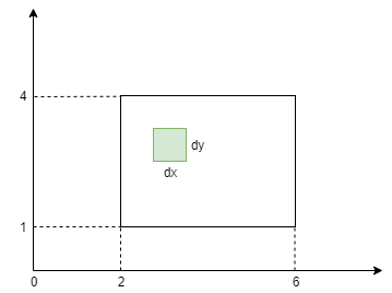
So, let’s start with computing the area of a rectangle using integration. Here, we define a rectangle in Catesian coordinates. We identify a small patch with length $dx$ and height $dy$. The area of this patch is $dx.dy$. Since there are 2 variables, we need to compute a double integral for the range of $x$ and $y$ respectively.

$$RectangleArea = \int_{x=2}^6\int_{y=1}^4dxdy = \int_{x=2}^6dx\int_{y=1}^4dy = \Big[x\Big]_{x=2}^6 \Big[y\Big]_{y=1}^4 = (6-2)(4-1) = 12$$

This checks out since the area of the rectangle for length 4 and height 3 is 12.

Next up, let’s try to compute the area of a circle of radius $R$ below.

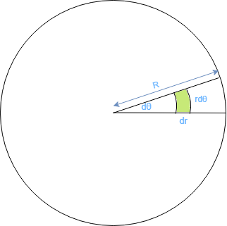
We similarly isolate a small pathch for integration. The length of the patch is a tiny segment along the radius $dr$. Computing the arc length of the patch is sligtly tricky. We need to somehow find a way to represent it in terms of the angle $d\theta$ represented in radians. Fortunately for us, there is a direct relationship between radians and the length of the arc that subtends that angle. [link]

So, the length of the arc is $rd\theta$. But what is the area of the patch? Turns out we can straighten the arc into a straight line, thereby converting our curved patch into a rectangle. This is known as rectification.

With that out of the way, the area of the patch can be simply represented by $dr.rd\theta$. Now, let’s find the area of the circle via integration.

$$CircleArea = \int_{r=0}^R\int_{\theta=0}^{2\pi}rd\theta dr = \int_{r=0}^Rrdr\int_{\theta=0}^{2\pi}d\theta = \Big[\frac{r^2}{2}\Big]_{r=0}^R \Big[\theta\Big]_{\theta=0}^{2\pi} = \Big(\frac{R^2}{2}\Big)(2\pi) = \pi R^2 \checkmark$$

Hemisphere Integration

With that out of the way, let’s get back to solving equation $(2)$. Here, we have to compute an itegral over the hemisphere.

$$\int_{\Omega}(\omega_i . n) d\omega_i$$

Like earlier, we have to identify a small patch that we can integrate on. For that we resort to spherical coordinates.

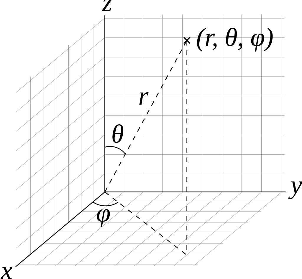
Here,
$\phi$ is known as the azimuth angle and its range is from $0$ to $2\pi$.
$\theta$ is known as the elevation angle and its range is from $0$ to $\frac{\pi}{2}$.

The following diagram shows us how such a patch can be constructed. The $rd\theta$ term is same as earlier since it lies on the great circle or meridian. The radius of other circle is smaller – $rsin\theta$. Hence, the length of that arc is $rsin\theta d\phi$ as shown below.

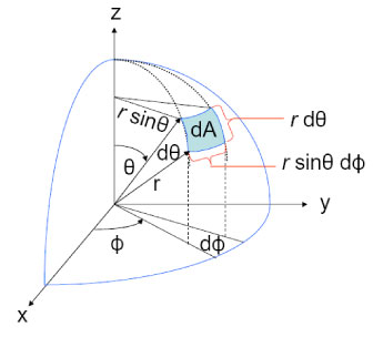
Since the direction vector $\omega_i$ and normal $n$ are assumed to be unit length, and the weakening factor is invariant to the azimuth angle, we can rewrite $\int_{\Omega}(\omega_i . n) d\omega_i$ as

$$\int_{\Omega}cos\theta d\omega_i = \int_{\theta=0}^{\frac{\pi}{2}}\int_{\phi=0}^{2\pi}cos\theta.rd\theta.rsin\theta d\phi =r^2 \int_{\theta=0}^{\frac{\pi}{2}} sin\theta cos\theta d\theta \int_{\phi=0}^{2\pi}d\phi$$

Using trigonometric identity $sin(2\theta) = 2sin \theta cos \theta$, and substituting $r=1$ for unit hemisphere, we can rewrite this as

$$\int_{\theta=0}^{\frac{\pi}{2}} \frac{sin2\theta}{2} d\theta \int_{\phi=0}^{2\pi}d\phi$$

Substituting, $\Theta = 2 \theta$ such that $\frac{d \Theta}{d \theta} = 2$, we can again rewrite this as

$$\int_{\Theta=0}^{\pi} \frac{sin\Theta}{2} \frac{d\Theta}{2} \int_{\phi=0}^{2\pi}d\phi = \frac{1}{4}\Big[-cos\Theta \Big]_{\Theta=0}^{\pi}\Big[\phi \Big]_0^{2\pi} = \frac{1}{4}\times2\times2\pi$$

Thus,

$$\int_{\Omega}cos\theta d\omega_i = \pi$$

and from equation $(2)$, we have

$$f_{lambert} = \frac{albedo}{\pi}$$

Hope you enjoyed this post. To understand its implications in lighting calculations check out this post by Sébastien Lagarde - Pi or not to Pi in game lighting equation.